[back to blog]

Extracting 3D parametric curves from 2D images of helical objects

Chris Willcocks, Philip Jackson, Carl Nelson, and Boguslaw Obara

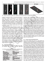
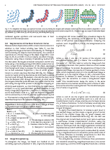
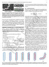
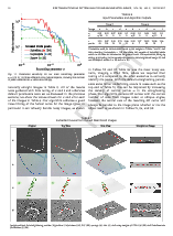
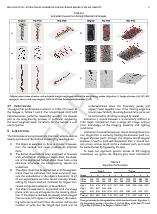
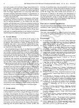
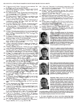
Click to go to full publication on IEEE Xplore.

Abstract

Helical objects occur in medicine, biology, cosmetics, nanotechnology, and engineering. Extracting a 3D parametric curve from a 2D image of a helical object has many practical applications, in particular being able to extract metrics such as tortuosity, frequency, and pitch. We present a method that is able to straighten the image object and derive a robust 3D helical curve from peaks in the object boundary. The algorithm has a small number of stable parameters that require little tuning, and the curve is validated against both synthetic and real-world data. The results show that the extracted 3D curve comes within close Hausdorff distance to the ground truth, and has near identical tortuosity for helical objects with a circular profile. Parameter insensitivity and robustness against high levels of image noise are demonstrated thoroughly and quantitatively.

Overview

In this paper, we take a 2D image of a helical object and automatically fit a 3D curve to it. To do this, we first segment and straighten the helical object and then we find peaks on the boundaries of the helical object. The curve fits through these peaks.

Applications

The primary applications of this research are to retrieve a 3D model of 2D images of helical objects, e.g. for collecting measurements, where 3D imaging is currently too expensive or impossible.

At a micro scale:

• Biology and medicine (e.g. Spirulina, Spirochaetes, sperm, bacterial macrofibers, microtubules, keratin, DNA, dynamin).
• Nanotechnology (e.g. helical nanostructures, such as: nanosprings and graphitic carbon microtubules).

At a macro scale:

• Medicine (e.g. umbilical cord).
• Biology (e.g. climbing plants, twining vines, twisted trees, seashells, Arabidopsis root).
• Cosmetics industry (e.g. hair).
• Engineering (e.g. screws, coils, springs, synthetic fiber ropes).

Areas for Future Research

To our knowledge, this is the first work that can automatically and robustly fit a 3D parametric curve to a single 2D image of a helical object. We believe there are several areas for improvement:

• In the future, a simpler algorithm for fitting 3D parametric curves to noisy 2D data will be found that doesn't require the straightening process. This will be faster and more robust, without the need for several parameters.
• The future research should focus on robustly capturing 2D polylines from 2D images and transforming the polyline geometry to capture the 2D helical structure. Extending the 2D polyline to a 3D piecewise helix is a well-researched area with good solutions.

Code Usage

Our code is written in MATLAB. To use it, clone the github repository somewhere and add it to your MATLAB workspace, then simply edit the image, set the parameters and run the script main.m.

I = imread('leptospira.png');
if (size(I,3) > 1); I = rgb2gray(I); end;                                   fprintf('\tdone!\nSegmenting...');

% Adjust algorithm parameters (see paper for detailed explanations)
straighten  = true;
sigma       = 0.01;             % smoothing amount, try 0.15 for 'licerasiae.png'
d           = max(size(I))/20;  % minimum distance between peaks, set to 0 for images with lots of coils
delta       = 50;
omega       = max(size(I))/20;
omicron     = 30;
push        = true;

% Run our algorithm steps
[c,B]       = part1_segment(I);                                             fprintf('\t\tdone!\nStraightening... ');
[Bp,T]      = part2_straighten(B,c,delta,omega,omicron,straighten);         fprintf('\tdone!\nFitting... ');
[p]         = part3_fitting(Bp,sigma,d,push);                               fprintf('\t\t\tdone!\nUndo transforms... ');
[tp]        = part4_undo_transforms(p,T,straighten);                        fprintf('\tdone!\n');

% Create our cubic spline (cs) through the transformed curve control points tp
cs = cscvn(tp);
cs = fnplotdense(cs);

% We can also use the straight spline (ss) from control points p
ss = cscvn(p);
ss = fnplotdense(ss);

% Example 3D metrics from the straight spline
tortuosity  = sum(sqrt(sum(diff(ss,1,2).^2,1))) / sqrt(sum((ss(:,end) - ss(:,1)).^2));
peaks       = floor(length(p)/2);

Citation

Please cite our paper:

@article{willcocks-2016-extract-3d-curve,
  author   = {C. Willcocks and P. Jackson and C. Nelson and B. Obara},
  journal  = {IEEE Transactions on Pattern Analysis and Machine Intelligence},
  title    = {Extracting 3D Parametric Curves from 2D Images of Helical Objects},
  year     = {2016},
  volume   = {PP},
  number   = {99},
  pages    = {1-1},
  doi      = {10.1109/TPAMI.2016.2613866},
  ISSN     = {0162-8828},
  month    = {},
}
  

[return to top]