October 2026. I design these practicals to keep iteration times short, so students see results and feel rewarded quickly. In our undergraduate and postgraduate practicals, each student gets an isolated Multi-Instance GPU (MIG) slice of an 80 GB NVIDIA A100: roughly 1/7 of its compute resources and 10 GB of dedicated GPU memory. In practicals 5–9, we train small models from scratch in minutes: a GPT on Shakespeare following Karpathy’s nanoGPT, image diffusion on CIFAR-10 horses, audio flow matching on a few AudioMNIST voices, and implicit video networks.
GPT from scratch
Building a GPT in plain PyTorch connects byte tokens and causal attention to next-token prediction. An excerpt generated by the teaching model after a couple of minutes of training on a student’s A100 share: [another sample]
ROMEO:
 that he had served up his world sons and ourselves!

ROMEO:
Why, now what she did not wear them but spent?
Image diffusion
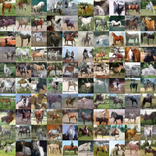
A small diffusion model learns to turn noise into images using only the horse class of CIFAR-10. Training the teaching model and generating these samples also takes a couple of minutes on a student’s A100 share.
Audio flow matching
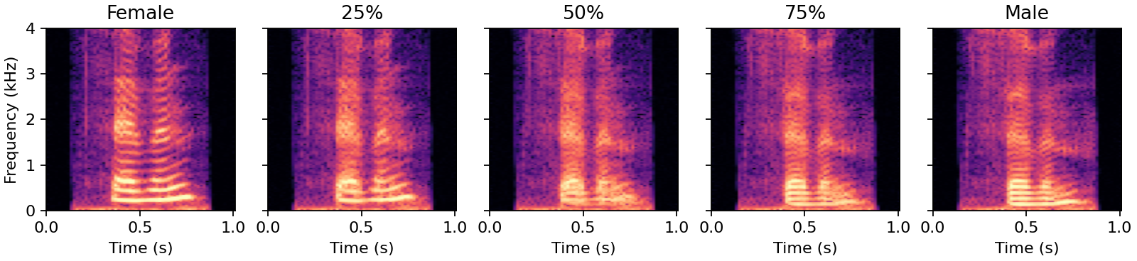
Generate speech from noise, then interpolate between female and male voices. Holding the initial noise fixed lets students hear the effect of changing the conditioning. These are five versions of “seven”.
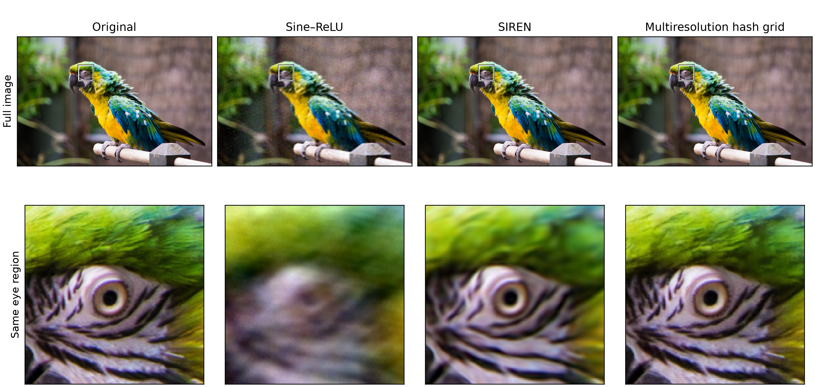
A network can represent an image by mapping a position to a colour. Below, Sine–ReLU, SIREN and multiresolution hash grids each fit the same image using less than 1 MiB. The enlarged eye makes the effect of the representation easy to see.
Cat video reconstruction
Original video alongside ReLU and multiresolution hash-grid reconstructions. Both fitted models use less than 1 MiB.
OriginalReLUHash grid
Bach reconstruction
A single network reconstructs this Bach recording by mapping time to amplitude. The fitted hash-grid model uses less than half a MiB.
Original
Network reconstruction
Images, audio and video share the model design, with weights fitted separately for each signal.
Each environment is a standalone .py file using PyTorch and the standard library. No Gymnasium: students can read and change the physics, observations, actions and rewards in one place.
Bandits
Inspect estimates and true rewards.
Compare the estimates with each arm’s true reward. (larger view)
Answers 1: Sample answers for some of the tasks in practical 1. (pdf)
Answers 1: Sample answers for some of the tasks in practical 2. (pdf)
Answers 3: Sample answers for some of the tasks in practical 3. (pdf)
All the above lecture material is made available under the CC-BY-NC-4.0. Some content within the lectures is from third parties and not covered by the license. Reference as follows, e.g. for DL and RL:
@misc{willcocks2021lectures,
  author       = {Chris G. Willcocks},
  title        = {Lectures on Deep Learning and Reinforcement Learning},
  year         = {2021},
  howpublished = {\textsc{url:}~\url{https://cwkx.com/blog.html#course-materials}}
}
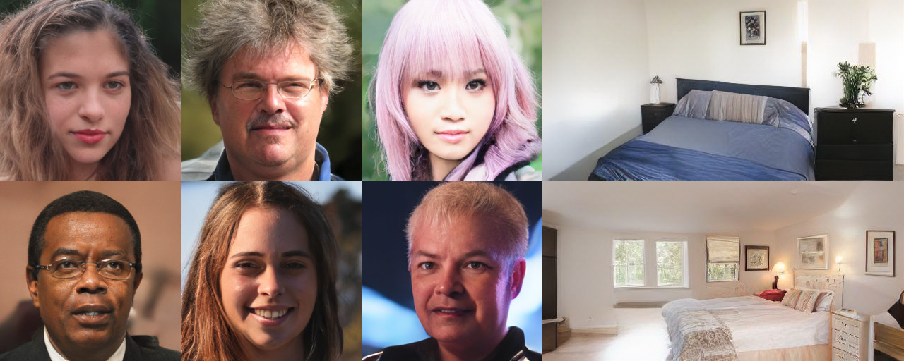
2022 · ECCV. Generating an image one token at a time is slow. We use discrete absorbing diffusion to predict many tokens in parallel, working with the compact codes of a vector-quantized image model.
The model also supports inpainting and outpainting, including generating images larger than those used during training. More examples and the method.
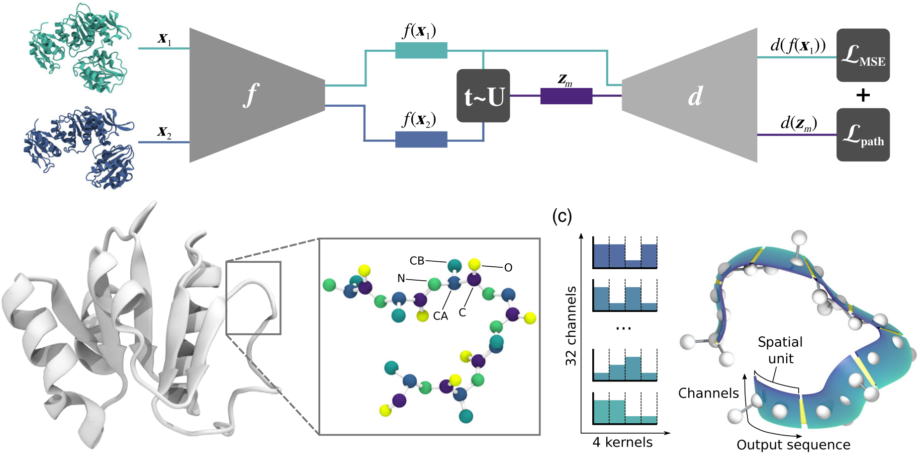
2021 · Physical Review X. Knowing a protein’s stable structures does not tell us how it moves between them. We combine molecular simulation with a convolutional network to learn a continuous space of conformations.
Physical constraints guide the intermediate structures. A model trained on distinct states can recover a biologically relevant transition path without being given examples along that path. Read the research write-up.
2021 · ICLR. Can a generative model learn a latent representation with only a decoder? Gradient origin networks start a latent vector at zero and use the gradient of the reconstruction loss as its encoding.
These videos show spherical interpolations through the learned latent spaces:
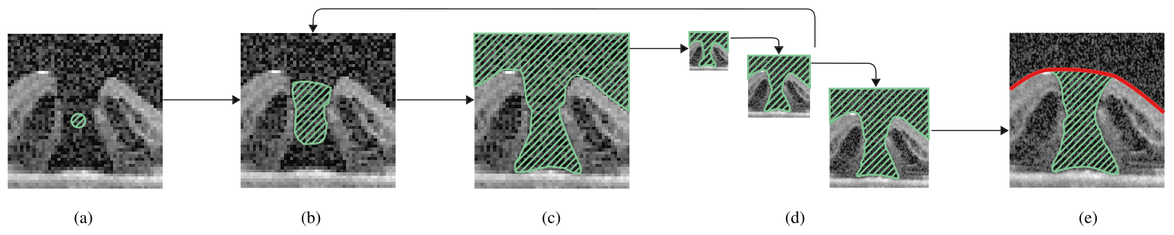
2018. OCT scans capture the three-dimensional shape of a macular hole, but manual measurements are often taken in two dimensions. Our method segments the full volume and fits surfaces to measure its area, height and diameters automatically.
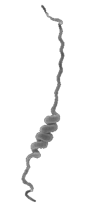
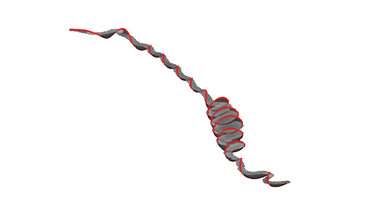
2016. Helical structures appear in bacteria, hair, springs and climbing plants. We recover a three-dimensional parametric curve from a single image by straightening the object, finding peaks along its boundary and fitting a helix through them.
The resulting curve lets us measure pitch, radius, length and tortuosity when three-dimensional imaging is impractical. Method, examples and code.
2013. My thesis explored rendering large scenes of animated voxel models. A CUDA renderer paged sparse voxel octrees through memory at the resolutions needed, using instancing and occlusion culling to keep the scene manageable.
Deformation exposed some interesting limitations, especially filling gaps left by forward transformations. The write-up also discusses later experiments with implicit surfaces and smooth blending. Thesis notes and figures.
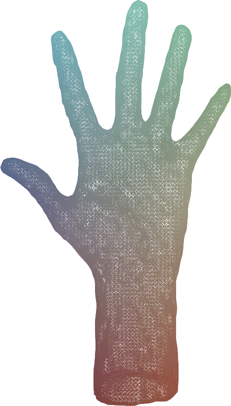
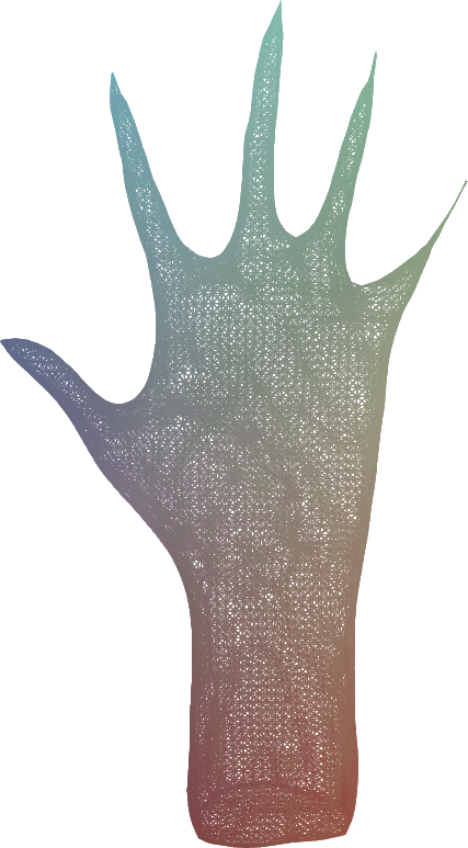
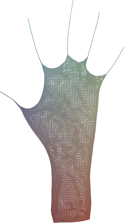
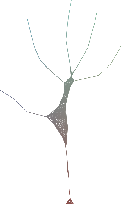
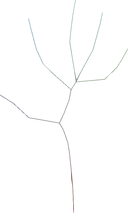
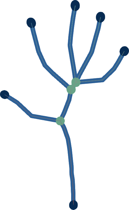
2012. A useful animation skeleton need not retain every small feature of a mesh. This method uses a target feature size to smooth away small details while retaining the larger structures as bones.
Two simple operations—smoothing neighbouring vertices and merging nearby vertices—contract the mesh into a skeleton. One parameter controls the scale of features that survive. How it works, and its limitations.